The derivative is the slope of the tangent line to the graph of a function. Hence, the sign of the derivative at a point tells us whether the function is increasing or decreasing there and how rapidly. We can use this to figure out essential features of a function and to sketch its graph.
Example 2.28 Let us try to figure out the behavior of the rational function

To begin with, a rational function is in trouble when the denominator is zero. Hence, the domain of this function does not include the point x = −1. Since the numerator is negative for x = −1, we can see that

The function is not continuous at x = −1. It is also easy to see that the function is zero when x = 1; there, the function crosses the horizontal axis. Another feature which is worth noting is the behavior for very large values of x, where x dominates the constants −1 and +1 at numerator and denominator, respectively:

To see the rate of increase/decrease of the function, we need its derivative. Applying the rule for the ratio of functions, we obtain

We see that the derivative is always positive, and it goes to +∞ when x tends to −1, both from the left and from the right.
Putting everything together, we see that this function:
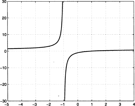
- Tends to 1 (from above) for x → −∞
- Increases on the interval (−∞, −1) and goes to +∞ when x approaches −1 from the left
- Goes to −∞ when x approaches −1 from the right
- Increases on the interval (1, ∞)
- Has value 0 for x = 1
- Tends to 1 (from below) for x → +∞
On the basis of these features, we could sketch a plot like Fig. 2.21.
As a more useful example, we are now able to figure out the behavior of the total cost function in the EOQ model of Section 2.1.
Example 2.29 The average total cost per unit time in the EOQ model is given by function

The last term does not depend on the order quantity Q, and its effect is to shift the graph up a bit. The linear component hQ/2 goes to zero for small order sizes and goes to +∞ for large order sizes. The nonlinear component Ad/Q goes to zero for large order sizes and goes to +∞ for small order sizes. Hence, we obtain

Fig. 2.21 Graph of the function of Example 2.28.

The domain of interest is the interval of strictly positive order quantities, (0, +∞). Unlike the rational function of the previous example, there is no point at which the function goes into trouble (is discontinuous) within this domain. Hence, it must be the case that the function is decreasing first, and then starts to increase.17 Indeed, the derivative is

Note that the constant term cd disappears in the derivative. Solving for Q, we see that the derivative is zero for

For Q < Q*, the derivative is negative and the function is decreasing. At point Q = Q*, the slope of the tangent line is horizontal. For Q > Q*, the derivative is positive and the function is increasing. This results in the plot of Fig. 2.2.
Since the total cost function is decreasing on interval (0, Q*) and increasing on interval (Q*, +∞), it must be the case that Q* is the optimal order size. This point is associated with a horizontal tangent line and we have good reasons to guess that such stationarity points are essential when optimizing a function.
DEFINITION 2.10 (Stationarity point) Given a function f(x), a point x* such that f′(x*) = 0 is called a stationarity point for the function. We also say that f is stationary at x*.
The EOQ example suggests that a function can be optimized by finding a stationarity point. In fact, life is not that easy, as many things can go wrong.
- To begin with, the function that we want to optimize may fail to be differentiable; for instance, the nondifferentiable function illustrated in Fig. 2.19(a) is minimized just where the derivative is not defined.
- Moreover, even if we assume continuity and differentiability, a stationarity point may be a minimum, a maximum, or neither. We are in trouble when functions oscillate; to see such examples, please take a look back at Fig. 2.8.
- Last but not least, a stationarity point might just be a local rather than a global optimum.
In order to better characterize points at which a function is maximized or minimized, we need some information that is not really provided by the derivative; we need information about the curvature of the function. This information is provided by second-order derivatives.
Leave a Reply