The role of convexity

Convexity and concavity play a major role in optimization. Consider a one-dimensional optimization problem, ; this problem is unconstrained, since x can be any point on the real line. Furthermore, assume that f is convex on the whole real line  and that x* is a stationarity point. Property 2.18 applies to x*:

for any , but this implies that x* is a global minimizer. We have proved the following theorem.

THEOREM 2.20 If function f is convex and differentiable on , then stationarity is a necessary and sufficient condition for global optimality in an unconstrained minimization problem. If f is concave, the result applies to an unconstrained maximization problem.

Example 2.35 The theorem above applies to an unconstrained optimization problem. If there are constraints, stationarity need not be associated with optimality. To see this, consider the minimization problem

The function f(x) = x² is convex, but it is easy to see that the minimizer is x* = 2, which is not a stationarity point. We need some more theory to cope with constrained problems. However, it may be the case that a constraint is nonbinding where the function is stationary and we find the minimizer by setting first-order derivative to zero. This happens, for instance, for the problem

Here the feasible region is [−2, +∞) but the constraint is nonbinding at stationarity point x* = 0, which is indeed the global minimizer. We speak in this case of an interior solution, as the minimizer lies in the interior of the feasible region.

We may also note that, since the second-order derivative of a convex function is always positive by property 2.19, then we do not run the risk of mistaking a maximum for a minimum. This, per se, does not imply global optimality, however. Still, property 2.19 is important because it provides us with an easy criterion to check convexity.

Example 2.36 Consider function

Its second-order derivative is f″(x) = 2b/x³, which is positive on the domain x > 0, if b > 0. Indeed, this is the case for the total cost function of the EOQ model, where b = Ad is the product of demand rate and fixed ordering charge, and we are interested in strictly positive order quantities. Hence, stationarity is in fact a necessary and sufficient condition for a globally optimal solution of the EOQ problem, which turns out to be an interior solution.

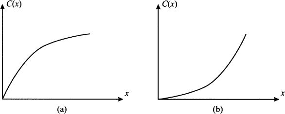
Apart from optimization, convexity and concavity are useful for characterizing functions that model essential features of a problem from an economic perspective. Consider a cost function c(x), quantifying the cost of some activity that we carry out at level x; this could be the cost of purchasing an item, but also the cost of producing an amount x of it. Two such functions are illustrated in Fig. 2.30. Both functions are increasing, as expected, but they are qualitatively different. In case (a) we see that the first-order derivative of the cost function is decreasing, whereas it is increasing in case (b). In economics, the first-order derivative of a cost function, evaluated at some point, is called the marginal cost. The marginal cost tells us the rate at which a cost is increasing when we raise the level x of the activity we are engaged in. For concave cost function (a), the marginal cost is decreasing; this implies that there is an economy of scale. On the contrary, convex function (b) models a diseconomy of scale, which may occur if the production process is less and less efficient when production volume is increased.

Fig. 2.30 Schematics of economies and diseconomies of scale.

We will see other uses of convexity and concavity, which are just worth mentioning here:

• We illustrate constrained optimization problems such asAs it turns out, a problem like this is relatively easy to solve if the feasible set S and the objective function f are both convex. If we are dealing with a maximization problem, it is easy if the function f is concave and the set S is convex.
• We deal with decision under uncertainty. In that setting, risk aversion of the decision maker plays a prominent role. We will see that one way of capturing risk aversion is by modeling preferences of the decision maker by a concave utility function.