The sample mean plays a key role in descriptive statistics and, as we shall see, in inferential statistics as well. In this section we take a first step to characterize its properties and, in so doing, we begin to appreciate an often cited principle: the law of large numbers.

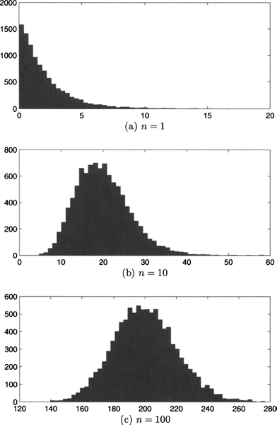
Fig. 7.22 Histograms obtained by sampling the sum of n independent exponentials with rate λ = 0.5, for n = 1,10,100.
Consider a sample consisting of i.i.d. variables Xi, i = 1,…,n, with expected value μ and variance σ2. The sample mean

is a random variable and it is natural to wonder what is its distribution. From what we have seen, we know that a general answer does not exist. However, if the sample comes from a normal population, the sample mean is normally distributed, because the sum of normals is normal as well. Furthermore, we can rely on the central limit theorem to conclude that sample mean will tend to be normal when the sample is large enough.
Another intuitive property of the sample mean is that it should get closer and closer to the true expected value μ, when n progressively increases. Indeed, on the basis of the properties of sums of random variables, we obtain

Furthermore, relying on the independence assumption, we also see that

This is a remarkable result: The larger the sample size, the lower the variance of the sample mean. In the limit, this variance goes to zero; but a random variable with zero variance is just a number. Then, we may suspect that we should write something like this:

This gets close to a precise statement of the law of large numbers. Actually, stating this law precisely requires to specify all of the hidden assumptions as well. Furthermore, the limit above has no clear meaning: What is the limit of a sequence of random variables? How can a random variable tend to a number? A sound statement of the law of large numbers requires some concepts of stochastic convergence. We will outline these concepts in the advanced Section 9.8; however, most readers may skip the involved technicalities.
Leave a Reply