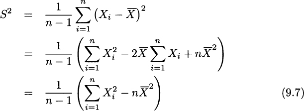
The typical estimator of variance is sample variance:

This formula can be understood as a sample counterpart of the definition of variance: It is basically an average squared deviation with respect to sample mean. When doing calculations by hand, the following rearrangement can be useful:

The sample standard deviation is just S, the square root of sample variance. We recall from Example 4.13 that rewriting variance like this may result in bad numerical behavior with some peculiar datasets; nevertheless, it is quite convenient in proving useful relationships.
An obviously weird feature of sample variance is that we take an average of n terms, yet we divide by n − 1. On the basis of the limited tools of descriptive statistics there is no convincing way of understanding why, when dealing with a population, we are told to divide by n, whereas we should divide by n − 1 when dealing with a sample. The right way to appreciate the need for this correction is to check for unbiasedness of sample variance.
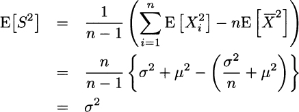
THEOREM 9.3 Sample variance is an unbiased estimator of true variance, i.e., E[S2] = σ2.
PROOF In the proof, we exploit rewriting (9.7) of sample variance:

In the second line above, we applied the usual property, Var(Y) = E[Y2] − E2[Y], to each Xi in the sum and to the sample mean ![]() .
.
To fully understand the result, observe that

but

In the second case, we should not divide by n when measuring deviations against ![]() rather than μ, and this results in a bias that is corrected by the n − 1 factor. From an intuitive perspective, we could say that the need to estimate the unknown expected value implies that we “lose one degree of freedom” in the n available data in the sample.
rather than μ, and this results in a bias that is corrected by the n − 1 factor. From an intuitive perspective, we could say that the need to estimate the unknown expected value implies that we “lose one degree of freedom” in the n available data in the sample.
Finding the expected value of sample variance is fairly easy, but characterizing its full distribution is not. One simple case is when the sample is normal. Intuitively, we see from Eq. (9.7) that sample variance involves squares of normal variables. Given what we know about the chi-square and Student’s t distribution, 5 the following theorem, which summarizes basic results on the distribution of the estimators that we have considered, should not come as a surprise.6
THEOREM 9.4 (Distributional properties of sample statistics) Let X1,…, Xn be a random sample from a normal distribution with expected value μ and variance σ2. Then
- The sample mean
 has normal distribution with expected value μ and variance σ2/n.
 - The random variable (n − 1)S2 / σ2 has chi-square distribution with n − 1 degrees of freedom.
- Sample mean and sample variance are independent random variables.
- The random variable
 has t distribution with n − 1 degrees of freedom.
Statement 1 is quite natural, since we know that the sum of jointly normal variables is itself a normal variable. Statement 2 can be understood by noting that in the sample mean we square and sum independent normal variables and recalling that by squaring and summing independent standard normals we get a chi-square; the distribution has n − 1 degrees of freedom, which is also reasonable, given what we observed about sample variance. Statement 3, on the contrary, is somewhat surprising, since sample mean and sample variance are statistics depending on the same random variables, but it is essential in establishing the last distributional result, which will play a fundamental role in the following. We should note that if the true variance were known, we could work with the statistic

which is a standard normal. If the random sample is not normal, the results above do not hold. Indeed, many results that are routinely used in inferential statistics are valid only for normal samples. Luckily, variations on the theme of the central limit theorem provide us with asymptotic results, i.e., properties that apply to large samples. These results justify the application of statistical procedures, which are obtained for normal samples, to large nonnormal samples. In what follows, we will rely on these procedures,7 but it is important to keep in mind that they just yield approximated results, and that due care must be exercised when dealing with small samples.
Leave a Reply