Production planning with assembly of components

The naive production mix model is just a starting point in modeling production planning, as many issues that make real-life models interesting and challenging are blatantly disregarded. We will proceed step by step, showing how more realistic features may be represented. In this section we consider one such issue, related to purchasing raw materials or manufacturing intermediate components. In fact, the product mix model directly relates demand to manufacturing of items; this means that we are disregarding the possible presence of components and subassemblies. As an example, let us consider how to generalize the product mix model to a two-level assembly-to-order (ATO) model. In an ATO system, we do not produce end items directly. First we make (or buy) modules; then, modules and components are assembled into end items. If manufacturing such modules requires a relatively long lead time, production decisions should be based on forecasted demand. Only when demand for end items is realized (i.e., customer orders are received) is assembly started. An ATO system is two-level in the sense that we have production to stock for modules, before demand is known, and assembly to order for end items. The strategy makes sense when a huge variety of end items results from combining a relatively limited number of basic modules. The sheer number of possible combinations makes stocking end items impossible or way too costly, whereas the time needed to make modules prevents pure production to order. The idea is to exploit a risk pooling effect, by which demand for modules is much less uncertain than demand for end items. A quite familiar example of such a system may be observed when you order a pizza. The wide number of end items prevents preparing a pizza before receiving a customer’s order. However, there is a limited number of basic ingredients, which can be prepared in advance and kept ready for use. A more industrial example is car or PC (personal computer) assembly, at least for those producers that offer a large degree of customization as a competitive weapon.

A true appreciation of the ATO system can be obtained only when accounting for uncertainty, something. Yet, as a first step, let us consider an unrealistic case characterized by deterministic and known demand for end items. Following the drill we have described before, let us define the basic sets we need, and the respective indices. We have

• A set I of modules, indexed by i
• A set J of end items, indexed by j
• A set M of resources, indexed by m

The data we need to tackle the problem extend what we have seen in the product mix problem:

• We need the demand d_j for each end item in J; note that demand is given for end items, not modules.
• We need to know how end items are assembled starting from modules; this means that, in our two-level system, we must specify what in manufacturing parlance is the gozinto factor, i.e., the number g_ij of modules of type i ∈ I needed to assemble one end item of type j ∈ J. This is a very simple example of a bill of material (BOM); true BOMs may entail many more levels and hundreds, if not thousands, of components.
• On the economic side, we need to know at which price p_j we sell end items, and the cost c_i of each module. In the naive mix problem, these two pieces of information are somehow merged into a contribution to profit; but here we make separate production and assembly decisions, and their economic features should be kept apart. For the sake of simplicity, we disregard assembly cost.
• On the technological side, we need the availability of each resource class m ∈ M, as well as the amount r_im of resource m needed to produce one module i. In principle, we should also consider similar data for the assembly process. However, for an ATO system to be effective, assembly must be rather fast. Hence, we assume that assembly is never a bottleneck, or, in other words, that the capacity constraint for assembly will never be binding. Whenever we know that a constraint is redundant, there are at least a couple of reasons for not including it in the model. The first reason is that if a constraint is redundant, then we should eliminate it in order to speed up computation. Actually, state of the art solvers are able to preprocess a model formulation and to eliminate redundant constraints before starting the solution algorithm, but there is a second, and maybe more important reason to avoid useless constraint: Writing them requires collecting data, which is a costly and wasted effort.

Finally, we need to specify our decision variables:

• The amount of modules of type i that we produce is denoted by x_i.
• The amount of end items of type j that we assemble and sell is denoted by y_j.

Arguably, both decision variables should be restricted to integer values; for the sake of simplicity, we will assume that a continuous approximation is acceptable. It is important to stress that we are dealing with an unrealistic model, whereby demand is assumed certain. In real-life ATO systems, these two decisions are made at different time instants: We must plan production of module now, before we know actual demand; only after receiving customer orders do we start assembly. This will be essential later,¹⁶ when we show how to represent uncertainty in demand. Our first step toward the right direction is the following deterministic LP model:

The objective function (12.22) is the difference between revenue from selling end items and cost from manufacturing modules. Constraints (12.23) and (12.25) are essentially the same capacity and market limitations as in the naive optimal mix model. The only constraint worthy of comment is (12.24), which links the two sets of decision variables. By multiplying the number of assembled end items by gozinto factors, and summing over end item types, we obtain the number of modules of type i needed to support assembly; this number is constrained by the number x_i of available modules. The careful reader will notice that this constraint could be rewritten as an equality constraint, as we will certainly not produce more modules than necessary. This is true in the idealized deterministic model, but later we will see that this is not the case when demand uncertainty enters the stage. For now, it may be useful to consider a toy example and analyze its solution.

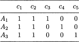
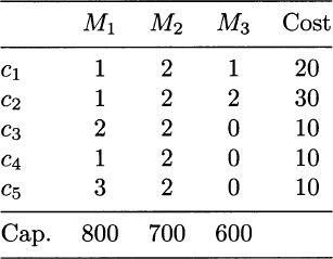
Example 12.10 To set up a small problem instance, say that we own a (very) small firm, producing just 3 end item types (A₁, A₂, A₃), which are obtained by assembling 5 component types (c₁, c₂, c₃, c₄, c₅). The components we use for each end item are described by a bill of materials, which is flat (just two levels: end items and components). The bill of materials is given in Table 12.1. Each entry in the table is a gozinto factor; for instance, to assemble an end item of type A₂, we need 1 component of type c₁, 1 of type c₂, and 1 of type c₄. From the bill of materials, we see that there are two common components, c₁ and c₂, while the remaining three are specific and characterize each end item. We assume that three resource types (M₁, M₂, M₃) are used for the production of components. Table 12.2 lists:

Table 12.1 Bill of materials for the assemble-to-order example.

Table 12.2 Bill of resources, cost of components, and available capacity (Cap.).

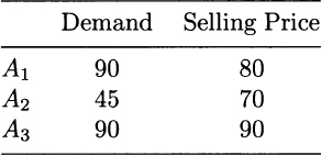
Table 12.3 Demand and selling price of end items.

• The bill of resources, i.e., the time required on each resource to manufacture one component.
• The available capacity for each resource class.
• The cost of each component; this cost might include both direct variable production costs and material costs. Since we assume that assembly is not a bottleneck, we do not list any resource consumption or capacity information concerning assembly.

We note that the cost of every end item type is 20 + 30 + 10 = 60; we do not make assembly cost explicit, but that would be easy to include. Other relevant data concern demand for end items and the price at which they are sold. They are given in Table 12.3. The last column displays the price at which end items are sold.¹⁷ For all of the three end items, the selling price is larger than 60, the total component cost; however, A₃ looks more profitable, because its contribution to profit is 90 − 60 = 30, whereas A₂ is the least profitable. We recall that this reasoning may be misleading, in that it does not take into account resource consumption. Solving the model, we obtain the following solution (rounded to 2 decimal digits):

The value of the objective function is 3233.33. In this very small example, we may easily interpret what this solution tries to accomplish. We assemble the maximum number of end items of type A₃, subject to its demand limitation d₃ = 90, since this is the most profitable one; this requires in turn the production of a corresponding number of common components c₁ and c₂, and of specific component c₅. Since the market limitation is binding for A₃, there is some capacity left, which is used to produce a limited amount of the specific component c₃, which is needed to assemble end item A₁, plus the corresponding number of common components. End item A₂ has the lowest selling price and is disregarded, as is its specific component c₄. It should be noted that, in general, one should not take for granted that the production of the highest profit item should be maximized; the consumption of available resources should be taken into account as well (as we learned by solving the production mix problem of Section 1.2).

The numerical solution of this toy example is very easy to interpret, but it should also be taken with utmost care. Any experienced production planner would be very critical about its “extreme” nature: It is essentially a bet on demand of the most profitable item. This might make sense if we are quite sure about demand, but what if actual demand turns out to be rather different? We might end up with a very large number of unused components, with a possible loss. The specific component c₅ of A₃ is risky, since demand for this item could be much lower than expected, but any remaining component of type c₅ cannot be used for anything else. To add insult to injury, if demand for A₃ is low but demand for other end items is high, we might lack specific components for A₁ and A₂. If so, we will be unable to use available common components as well. We need a way to obtain robust solutions when facing uncertain scenarios. In Section 13.3.1 we show one possible approach to accomplish this aim.