All well deliverability equations relate the well production rate and the driving force in the reservoir, that is, the pressure difference between the initial, outer boundary or average reservoir pressure and the flowing bottomhole pressure.
If the bottomhole pressure is given, the production rate can be obtained readily. However, the bottomhole pressure is a function of the wellhead pressure, which, in turn, depends on production engineering decisions, separator or pipeline pressures, and so on. Therefore, what a well will actually produce must be the combination of what the reservoir can deliver and what the imposed wellbore hydraulics would allow.
It is then useful to present the relationship between the well production rate and the bottomhole pressure as the inflow performance relationship (IPR). Usually, the bottomhole pressure, pwf, is graphed on the ordinate and the production rate, q, is graphed on the abscissa.
Equations (2-9), (2-26), and (2-44) can be used for steady-state, transient, and pseudosteady-state IPR curves. The following examples illustrate these concepts.
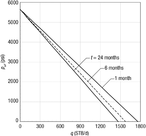
Using the well and reservoir data in Appendix A, construct transient IPR curves for 1, 6, and 24 months. Assume zero skin.
Solution
Equation (2-24) with substituted variables takes the form

The relationship between q and pwf of course will depend on time, t [which in Equation (2-50) must be entered in hours]. Figure 2-5 is a graph of the transient IPR curves for the three different times.

Figure 2-5. Transient IPR curves for Example 2-7.
Example 2-8. Steady-State IPR: Influence of the Skin Effect
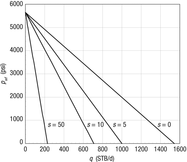
Assume that the initial reservoir pressure of the well described in Appendix A is also the constant pressure of the outer boundary, pe (steady state). Draw IPR curves for skin effects equal to 0, 5, 10, and 50, respectively. Use a drainage radius of 2980 ft (A = 640 acres).
Solution
Equation (2-9) describes a straight-line relationship between q and pwf for any skin effect. For example, after substitution of variables for a skin equal to 5, Equation (2-9) becomes

Similarly, the multipliers of the rate for the 0, 10, and 50 skin effects are 3.66, 7.67, and 23.7, respectively.
Figure 2-6 gives the steady-state IPR curves for the four skin effects.

Figure 2-6. Steady-state and impact of skin effect for Example 2-8.
Example 2-9. Pseudosteady-State IPR: Influence of Average Reservoir Pressure
This calculation is the most useful and the one most commonly done for the forecast of well performance. Each IPR curve reflects a “snapshot” of well performance at a given reservoir pressure. This is a time-dependent calculation, done in discrete intervals. Combination with volumetric material balances will allow the forecast of rate and cumulative production versus time.
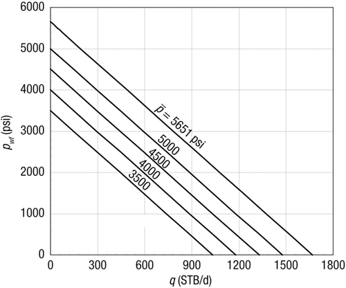
For this exercise, calculate the IPR curves for zero skin effect but for average reservoir pressures in increments of 500 psi from the “initial” 5651 to 3500 psi. Use all other variables from Appendix A. Drainage radius is 2980 ft.
Solution
Equation (2-44) is the generalized pseudosteady-state equation for any drainage shape and well position. For a circular drainage shape, Equation (2-34) is sufficient.
Substituting the variables from Appendix A into Equation (2-34) results (for ![]() ) in
) in

For all average reservoir pressures, the slope in Equation (2-51) will remain the same. The intercept will simply be the average pressure. Therefore, as shown in Figure 2-7, the pseudosteady-state IPR curves are depicted as parallel straight lines, each reflecting an average reservoir pressure.

Figure 2-7. Pseudosteady-state IPR curves for a range of average reservoir pressures (Example 2-9).
For these simplified examples, the slope of the IPR is the reciprocal of the productivity index, J.
Leave a Reply