Expected value and variance do not tell us the whole story about a random variable. To begin with, they do not say anything about the possible lack of symmetry. From descriptive statistics, we know that to characterize symmetry of a distribution, or lack thereof, we need a coefficient measuring its skewness. Furthermore, we may have distributions according to which extreme events, like huge losses due to a stock market crash, are pretty rare, and distributions in which they are not that unlikely. The probability of extreme realizations of random variables depends on the probability mass associated with the tails of the distribution. Needless to say, when dealing with risk management we do need measures taking these features into account. They all rely on the definition of a more general concept, moments of a random variable.
DEFINITION 7.3 (Moments of a random variable) The moment of order k of random variable X is defined as E[Xκ]. The central moment of order κ is defined as E[(X − μX)κ].
We immediately see that expected value is just the first-order moment, whereas variance is the second-order central moment. To characterize deviations with respect to the expected value, we need an even-order moment, to avoid can-celation between positive and negative deviations. But in order to capture lack of symmetry, we need just that, which is captured by a central moment of odd order. Furthermore, in order to capture fat tails, we need higher-order moments than just the second one. This motivates the following definitions.
DEFINITION 7.4 (Skewness and kurtosis) Skewness is defined as

Kurtosis is defined as

Looking at these definition, one could wonder why we should divide the moment of order k = 3,4 by a corresponding power of the standard deviation σ. The point is that the above properties should not depend on change of scale or shifts in the underlying distribution: If we define a random variable Y = α + βX, its skewness and kurtosis should be the same as X. It is easy to see that skewness is not changed by this linear affine transformation:

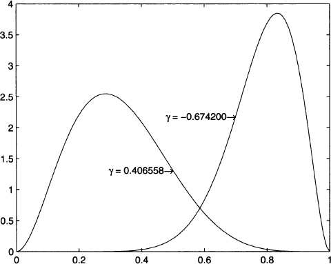
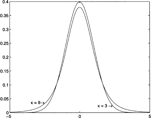
The same applies to kurtosis. In Fig. 7.9 we illustrate two asymmetric distributions. The PDF on the left is skewed to the right and has positive skew; in such a case, the median is smaller than the expected value. The PDF on the right is skewed to the left and has negative skew. Figure 7.10 shows two distributions with different tail behavior. The distribution with kurtosis κ = 9 has fatter tails and a corresponding lower mode. This makes sense, as the overall area below any PDF must always be 1; if tails are fatter, some probability mass is removed from the central portion of the distribution.

Fig. 7.9 Schematic representation of positive and negative skewness.

Fig. 7.10 Schematic representation of kurtosis.
Leave a Reply