A full characterization of discrete random variables can be given in terms of PMF or CDF. They are related, as the CDF can be obtained from the PMF by summing, and we can go the other way around by taking differences. For the reasons we have mentioned, in the continuous case the role of the PMF is assumed by a probability density function, whereas the CDF is defined in exactly the same way:2

As we have pointed out, the PDF is a nonnegative function fx(x) that does not give the probability of a single value, but can be used to evaluate probabilities of intervals:

Then, it is easy to see the link between PDF and CDF:

Since the PDF is nonnegative, the CDF is a nondecreasing function:

Furthermore

The last property is just another way to express the normalization condition on the PDF:

We may observe a few similarities between CDFs of discrete and continuous random variables:
- The CDF is a nondecreasing function ranging from 0 to 1.
- We obtain CDF by summing probabilities expressed by the PMF of discrete random variables, and by integrating the PDF of continuous random variables; since the integral is, in a sense, a sort of continuous sum, this is not surprising.
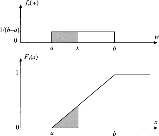
 Fig. 7.5 From PDF to CDF in the case of a uniform distribution.
The main difference is that, unlike the discrete case, the CDF of a continuous random variable is a continuous function, as illustrated in the following example.
Example 7.1 To illustrate the link between CDF and PDF, consider the PDF of a uniform distribution:

Clearly, the event {X ≤ a} has zero probability; hence, we should expect that FX(x) = 0 x ≤ a. Indeed

For a ≤ x ≤ b we have

Finally, FX(x) = 1 for x ≥ b. Both PDF and CDF of a uniform distribution are illustrated in Fig. 7.5.
From the example, we see that since the CDF is the integral of the PDF, it is a continuous function, even if the PDF has some kinky point. On the contrary, the CDF in the discrete case jumps because the probability mass is concentrated at a discrete set of points, rather than being distributed on a continuous support.
We may also better understand why the probability of any specific value is zero for continuous random variables:

As a consequence, in the continuous case, we obtain

Another point worth mentioning is that

As a final remark, we recall that in the discrete case we may go from CDF to PMF by taking differences. With continuous random variables, the equivalent operation is taking the derivative of the CDF. Indeed, we may also write P(a ≤ X ≤ b) as

which implies

Recalling the fundamental theorem of calculus,3 we conclude that

Leave a Reply