Central limit theorem

cAs we noted, it is difficult to tell which distribution we obtain when summing a few i.i.d. variables. Surprisingly, we can tell something pretty general when we sum a large number of such variables. We can get a clue by looking at Fig. 7.22. We see the histogram obtained by sampling the sum of independent exponential random variables with rate λ = 0.5 or, in other words, expected value 2; the sample size is 10,000. In plot (a) we see the histogram for just one exponential variable; we observe the exponential shape that we expect. Plot (b) shows the histogram when n = 10 independent exponentials are summed; finally, plot (c) shows what happens for n = 100. The last histogram looks suspiciously like a normal density. Indeed, the celebrated central limit theorem confirms the intuition.

THEOREM 7.9 (Central limit theorem) Let X₁, X₂, …, X_n be a sequence of i.i.d. random variables with expected μ and standard deviation σ.

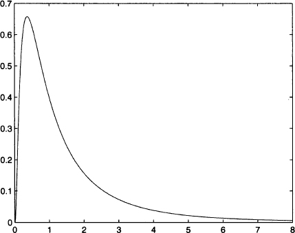
Fig. 7.21 PDF of a lognormal variable with parameters μ = 0 and σ = 1.

Then, for n large, the following holds:

where Z is standard normal.

This theorem essentially states that the sum of n i.i.d. variables tends to a normal distribution with expected value nμ and standard deviation ; by standardization we get Z.²³ The central limit theorem contributes to explain why the normal distribution plays a pivotal role: When we sum many random contributions, we tend to end up with a normal distribution. For instance, demand for items sold in high volumes can often be modeled by a normal distribution, resulting from the sum of many individual demands, whereas this model is inappropriate for low-volume items.