Options are financial derivatives that have gained importance, as well as a bad reputation, over the years. In Section 1.3.1 we considered forward contracts, another type of derivative. With a forward contract, two parties agree on exchanging an asset or a commodity, called the underlying asset, at a prescribed time in the future, for a fixed price determined now. In a call option, one party (the option holder, i.e., the party buying the option) has the right but not the obligation to buy the asset from the other party (the option writer, i.e., the party selling the option) at a price established now. This is called the strike price, which we denote by K. Let us denote the current price of the underlying asset by S0 (known when the option is written) and the future price at a time t = T by ST. Note that ST, as seen at time t = 0, is a random variable; the time t = T corresponds to the option maturity, which is when the option can be exercised.2 Clearly, the option will be exercised only if ST ≥ K, since there would be no point in using the option to buy at a price that is larger than the prevailing market price at time T. Then the payoff of the option, for the holder, is

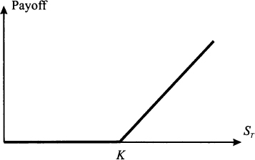
Fig. 3.1 Payoff of a call option.

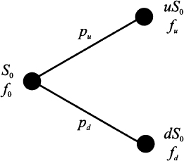
To interpret this, consider the possibility of exercising the option to buy at K an asset that can be immediately sold at ST. Market structure is not really that simple, but some options are settled in cash, so the payoff really has a monetary nature; this occurs for options written on a nontraded market index or on interest rates. This payoff is a piecewise linear function and is illustrated in Fig. 3.1. When the future asset price ST will be realized, at time t = T, the payoff will be clearly determined. What is not that clear is the fair price for the contract at time t = 0: The payoff for the option holder cannot be negative, but the option writer can suffer a huge loss; hence, the latter requires an option premium, paid at time t = 0, to enter into this risky contract. Here we consider the most elementary model for option pricing. Whatever model we may think of, it should account for uncertainty in the price of the underlying asset, and the simplest model of uncertainty is a binomial model.3 As shown in Fig. 3.2, a binomial model for the price of the underlying asset assumes that its price in the future can take one of two values. It is quite common in financial modeling to represent uncertainty using multiplicative shocks, i.e., random variables by which the current stock price is multiplied to obtain the new price. In a binomial model, this means that the current price S0, after a time period of length T, is multiplied by a shock that may take values d or u, with probabilities pu and pd, respectively. It is natural to think that d is the shock if the price goes down, whereas u is the shock when the price goes up; so, we assume d < u. The asset price may be either S0u or S0d, and the option will provide its holder a payoff fu and fd corresponding to the two outcomes. These values are also illustrated in Fig. 3.2. For instance, in the case of a call option with strike price K, we have

Fig. 3.2 One-step binomial model for option pricing.

The pricing problem consists of finding a fair price f0 for the option, i.e., its value at time t = 0. Intuitively, one would guess that the two probabilities pu and pd play a major role in determining f0 Furthermore, individual risk aversion could also play a role. Different people may assign a different value to a lottery, possibly making the task of finding a single fair price a hopeless endeavor, unless we have an idea of the aggregate risk aversion of the market as a whole.
However, a simple principle can be exploited in order to simplify our task. The option is a single, somewhat complicated, asset; now suppose that we are able to set up a portfolio of simpler assets, in such a way that the portfolio yields the same payoff as the option, in any possible future state. The value of this replicating portfolio at t = 0 is known, and it cannot differ from the option value f0. Otherwise, there would be two essentially identical assets traded at different prices. Such a violation of the law of one price would open up arbitrage opportunities.4
The replicating portfolio should certainly include the underlying asset, but we need an additional one. Financial markets provide us with such an asset, in the form of a risk-free investment. We may consider a bank account yielding a risk-free interest rate r; we assume here that this rate is continuously compounded,5 so that if we invest $1 now, we will own $ert at a generic time instant t. Equivalently, we may think of a riskless zero-coupon bond, with initial price B0 = 1 and future price B1 = erT, when the option matures at time t = T.
What we have to find is the number of stock shares and riskless bonds that we should include in the portfolio, in order to replicate the option payoff. Let us denote the number of stock shares by Δ and the number of bonds by Ψ. The initial value of this portfolio is

and its future value, depending on the realized state, will be either

Note that future value of the riskless bond does not depend on the realized state. If this portfolio has to replicate the option payoff, we should enforce the following two conditions:

This is a system of two linear equations in two unknown variables Δ and Ψ. The equations are linear as variables occur linearly. There is no power like x3, or cross-product like x1 · x2, or any weird function involved. All we have to do is solve this system of linear equations for Δ and Ψ, and plug the resulting values into Eq. (3.1) to find the option price f0. A simple numerical example can illustrate the idea.
Example 3.1 Let us assume that option maturity is T = 1 year, the risk-free interest rate is 10%, the current price of the stock share is $10, and the strike price is $11. Finally, say that the two possible returns of the stock share in one year are either 20% or −10%, which imply u = 1.2 and d = 0.9. The corresponding payoffs are

The system of linear equations is

If we subtract the second equation from the first one, we get

Plugging this value back into the first equation yields

and putting everything together, we obtain

Note that a negative value of Ψ means that we borrow some money, at the risk-free rate.
To get a financial understanding of what is going on, you should take the point of view of the option writer, i.e., the guy selling the option. Say that he takes a “naked” position, i.e., he collects the option price and waits until maturity. If the stock price goes up, he will have to buy one share at $12 just to hand it over to the option holder for $11, losing $1. If he does not like taking this chance, he could consider the opposite position: Buy one stock share, just in case the option gets exercised by its holder. This “covered” position does not really solve the problem, as the writer loses $1 if the price goes down, the option is not exercised, and he has to sell for $9 the share that was purchased for $10.
The replicating strategy suggests that, to hedge the risk away, the writer should actually buy ![]() shares. To this aim, he should use the option premium, plus some borrowed money ($2.7145, as given by Ψ). If the stock price goes down to $9, the option writer will just sell that share for $3, i.e., what he needs to repay the debt, which at the risk-free rate has risen to $3. Hence, the option writer breaks even in the “down” scenario. The reader is encouraged to work out the details for the other case, which requires purchasing two additional thirds of a stock share at the price of $12, in order to sell a whole share to the option holder, and to verify that the option writer breaks even again (in this case, the proceeds from the sale of the share at the strike price are used to repay the outstanding debt).
shares. To this aim, he should use the option premium, plus some borrowed money ($2.7145, as given by Ψ). If the stock price goes down to $9, the option writer will just sell that share for $3, i.e., what he needs to repay the debt, which at the risk-free rate has risen to $3. Hence, the option writer breaks even in the “down” scenario. The reader is encouraged to work out the details for the other case, which requires purchasing two additional thirds of a stock share at the price of $12, in order to sell a whole share to the option holder, and to verify that the option writer breaks even again (in this case, the proceeds from the sale of the share at the strike price are used to repay the outstanding debt).
This numerical example could leave the reader a bit puzzled: Why should anyone write an option just to break even? No one would, of course, and the fair option price is increased somewhat to compensate the option writer. Furthermore, we have not considered issues such as transaction costs incurred when trading stock shares. Most importantly, the binomial model of uncertainty is oversimplified, yet it does offer a surprising insight: The probabilities pu and pd of the up/down shocks do not play any role, and this implies that the expected price of the stock share at maturity is irrelevant. This is not surprising after all, as we have matched the option payoff in any possible state, irrespective of its probability. Moreover, the careful reader will recall that we reached a similar conclusion when dealing with forward contracts in Section 1.3.1. There, by no-arbitrage arguments that are actually equivalent to what we used here, it was found that the fair forward price for delivery in one year is F0 = S0(l + r), where S0 is the price of the underlying asset at time t = 0 and r is the risk-free rate with annual compounding. In the case of continuous compounding and generic maturity T, we get F0 = S0erT.
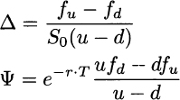
Let us try to see if there is some link between forward and option pricing. To begin with, let us solve the system of linear equations (3.2) in closed form. Using any technique described in the following section,6 we get the following composition of the replicating portfolio:

Hence, by the law of one price, the option value now is

As we already noticed, this relationship does not depend on the objective probabilities pu and pd. However, let us consider the quantities

which happen to multiply the option payoffs in Eq. (3.3). We may notice two interesting features of πu and πd:
- They add up to one, i.e., πu + πd = 1.
- They are nonnegative, i.e., πu, πd ≥ 0, provided that d ≤ erT ≤ u.
The last condition does make economic sense. Suppose, for instance, that erT < d < u. This means that, whatever the realized scenario, the risky stock share will perform better than the risk-free bond. But this cannot hold in equilibrium, as it would pave the way for an arbitrage: Borrow money at the risk-free rate, buy the stock share, and you will certainly be able to repay the debt at maturity, cashing in the difference between the matured debt and the stock price. On the contrary, if the risk-free rate is always larger than the stock price in the future, one could make easy money by selling the stock share short.7
We already know that probabilities may be related to relative frequencies and that the latter do add up to one and are nonnegative. Then we could interpret πu and πd as probabilities and Eq. (3.3) can be interpreted in turn as the discounted expected value of the option payoff

provided that we do not use the “objective” probabilities pu and pd, but πu and πd These are called risk-neutral probabilities, a weird name that we can easily justify. Indeed, if we use the probabilities πu and πd, the expected value of the underlying asset at maturity is

where the notation ![]() emphasizes that change in probability measure.8 This suggests that, under these unusual probabilities, the return of the risky asset is just the risk-free return. Furthermore, this is just the forward price of the underlying asset. In other words, the forward price is in fact the expected value of the underlying asset, but under modified probabilities. But how is it possible that the expected return of a risky asset is just the risk-free rate? This might happen only in a world where investors do not care about risk, i.e., in a risk-neutral world, which justifies the name associated with the probabilities we use in option pricing. Indeed, what we have just illustrated is the tip of a powerful iceberg, the risk-neutral pricing approach, which plays a pivotal role in financial engineering.
emphasizes that change in probability measure.8 This suggests that, under these unusual probabilities, the return of the risky asset is just the risk-free return. Furthermore, this is just the forward price of the underlying asset. In other words, the forward price is in fact the expected value of the underlying asset, but under modified probabilities. But how is it possible that the expected return of a risky asset is just the risk-free rate? This might happen only in a world where investors do not care about risk, i.e., in a risk-neutral world, which justifies the name associated with the probabilities we use in option pricing. Indeed, what we have just illustrated is the tip of a powerful iceberg, the risk-neutral pricing approach, which plays a pivotal role in financial engineering.
Of course, the binomial model we have just played with is too simple to be of practical use, but it is the building block of powerful pricing methods. We refer the interested reader to references but now it is time to summarize what we have learned from a general perspective:
- Building and solving systems of linear equations may be of significant practical relevance in many domains, including but not limited to financial engineering. We have already stumbled on systems of linear equations when solving the optimal production mix problem in Section 1.1.2.
- We have also seen an interplay between algebra and probability theory; quantitative, fact-based business management requires the ability of seeing these and other connections.
- We have considered a simple binomial model of uncertainty. We had two states, and we used two assets to replicate the option. What if we want a better model with three or more states? How many equations do we need to find a solution? More generally, under which conditions are we able to find a unique solution to a system of linear equations?
We will not dig deeper into option pricing, which is beyond the scope of the book, but these questions do motivate further study, which is carried out in the rest. But first, we should learn the basic methods for solving systems of linear equations.
Leave a Reply