A mean–risk formulation of the assembly-to-order problem

Mean–risk formulations are based on the idea of trading off expected profit (or return) against a risk measure. Classical mean–variance portfolio optimization relies on an analytical representation of variance, which leads to an easy convex quadratic programming problem. This need not be the case if we choose another risk measure. Value at risk is easy to evaluate and optimize under a normality assumption, but it may turn awkward in general, as its minimization may result in a nonconvex optimization problem. Conditional VaR is better behaved from this point of view, and it may lead to a (stochastic) linear programming model formulation.²² Hence, we may consider minimizing CVaR, at some confidence level 1 − α, subject to a constraint on expected profit or loss; by changing this target expectation, we may trace an efficient frontier of solutions.

Let f(x, Y) be a loss or cost function, depending on a vector of decision variables x and a vector of random variables Y with joint density g_Y(y), and consider function F_1−α(x, ζ) defined as

where [z]⁺ ≡ max{z, 0}, and  is an auxiliary variable. It can be shown that minimization of CVaR, at confidence level 1 − α, is accomplished by the minimization of F_1−α(x, ζ) with respect to its arguments. In a stochastic linear programming model based on discrete scenarios, if we denote by f(x, y^s) the loss in scenario s, s ∈ S, the minimization of CVaR is equivalent to the solution of the LP model

where π^s is the probability of scenario s ∈ S, subject to the additional constraints depending on the specific model.

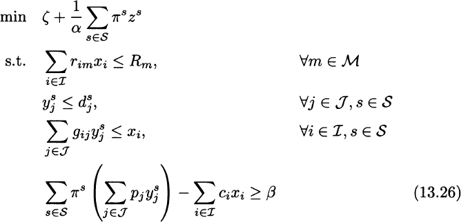
The application of this result to the ATO problem is rather straightforward:

Decision variables, parameters, and constraints have the same meaning as in the previous ATO models. The only constraint worth mentioning is Eq. (13.26), which sets a lower bound β on expected profit. Also note that we change the sign of profit in Eq. (13.27), which should refer to a loss function.