Boxplots

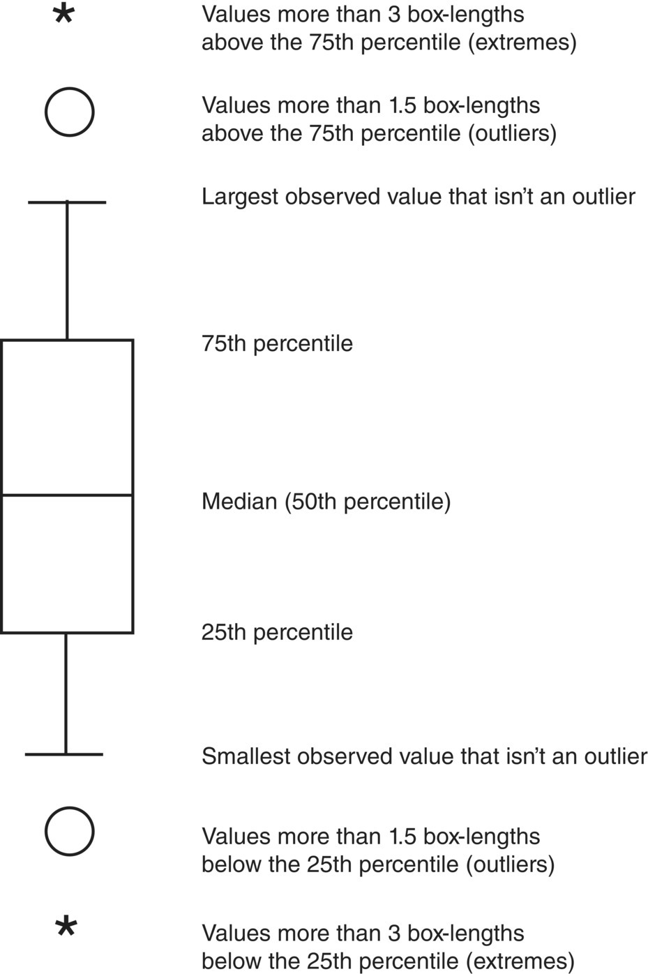
A display that further summarizes information about the distribution of the values is the boxplot. Instead of plotting the actual values, a boxplot displays summary statistics for the distribution. It is a plot of the 25th, 50th, and 75th percentiles, as well as values far removed from the rest.

Figure 8.2 shows an annotated sketch of a boxplot. The lowest boundary of the box is the 25th percentile. Tukey (1977) refers to the 25th and 75th percentile “hinges.” Note that the 50th percentile is the median of the overall data set, the 25th percentile is the median of those values below the median, and the 75th percentile is the median of those values above the median. The horizontal line inside the box represents the median. Of the cases, 50% are included within the box. The box length corresponds to the interquartile range, which is the difference between the 25th and 75th percentiles.

The boxplot includes two categories of cases with outlying values. Cases with values that are more than 3 box lengths from the upper or lower edge of the box are called extreme values. On the boxplot, these are designed with an asterisk (*). Cases with values that are between 1.5 and 3 box‐lengths from the upper or lower edge of the box are called outliers and are designed with a circle. The largest and smallest observed values that aren’t outliers are also shown. Lines are drawn from the ends of the box to these values. (These lines are sometimes called whiskers and the plot is then called a box‐and‐whiskers plot.)

Despite its simplicity, the boxplot contains an impressive amount of information. From the median you can determine the central tendency, or location. From the length of the box, you can determine the spread, or variability, of your observations. If the median is not in the center of the box, you know that the observed values are skewed. If the median is closer to the top of the box than to the bottom, the opposite is true: the distribution is negatively skewed. The length of the tail is shown by the whiskers and the outlying and extreme points.

EXAMPLE 8.6

Eighteen measurements of the disbursement rate (cm³/s) of a chemical disbursement system are recorded and sorted:

1. Compute the sample mean and sample variance.
2. Find the sample upper and lower quartiles.
3. Find the sample median.
4. Construct a boxplot of the data.
5. Find the 5th and 95th percentiles of the inside diameter.

SOLUTION

1. Sample mean: 8.059; Sample variance: 0.661
2. Q₁: 7.575, Q₃: 8.535
3. Sample median: 8.235
4. 5th percentile: 6.175; 95th percentile: 9.331.