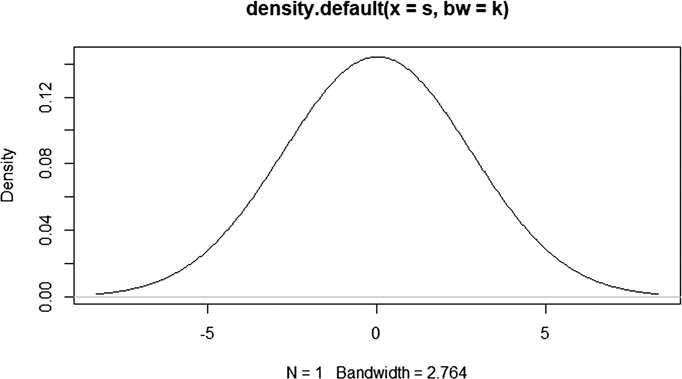
Figure 2.7 shows the skewness and kurtosis of the dataset. The skewness of the rainfall data is 0.01999941. It shows that the distribution of data is positively skewed. Kurtosis value is 2.763914. This is less than 3 which means the data contain low-level outliers.

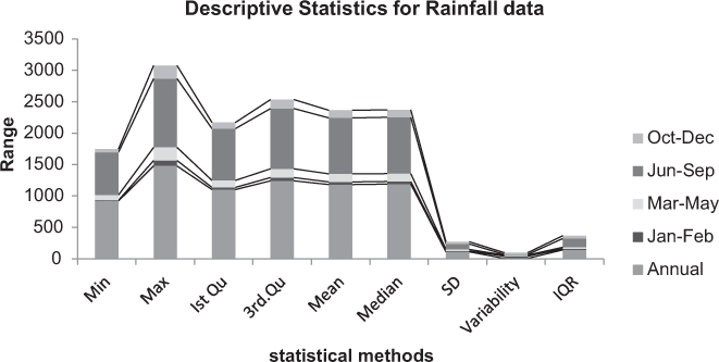
Table 2.3 explains the overall summary of data with parameters like minimum, maximum, mean, median, IQR, standard deviation values for the annual and seasonal rainfall (Figure 2.8).
| Minimum | Maximum | First quarter | Third quarter | Mean | Median | Standard deviation | Variability | IQR | |
|---|---|---|---|---|---|---|---|---|---|
| Annual | 920.8 | 1480.3 | 1102.4 | 1242.5 | 1182.0 | 1190.5 | 110.68 | 9.36 | 141.15 |
| January–February | 11.70 | 86.30 | 33.80 | 51.40 | 43.19 | 41.30 | 14.47 | 33.51 | 17.6 |
| March–May | 84.5 | 209.7 | 112.3 | 139.7 | 128.7 | 125.1 | 22.89 | 17.79 | 27.3 |
| June–September | 679.5 | 1094.5 | 823.5 | 959.6 | 890.3 | 897.8 | 89.17 | 10.01 | 136.1 |
| October–December | 52.7 | 207.50 | 97.05 | 142.15 | 119.88 | 116.20 | 32.46 | 27.08 | 45.1 |

Seasonal rainfall level:
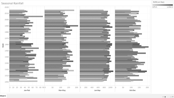
The seasonal rainfall level expresses the maximum rainfall that occurred in 1960 in the October–December interval. Based on the comparison of four seasons, June–September and October–December seasons faced high rainfall (Figure 2.9).

Leave a Reply